Session 7: How can I create new categorical variable?

A Slower Introduction to R

Yea-Hung Chen, PhD, MS

UCSF Library

Thursday, November 20, 2025

Reordering groups

Hypertension

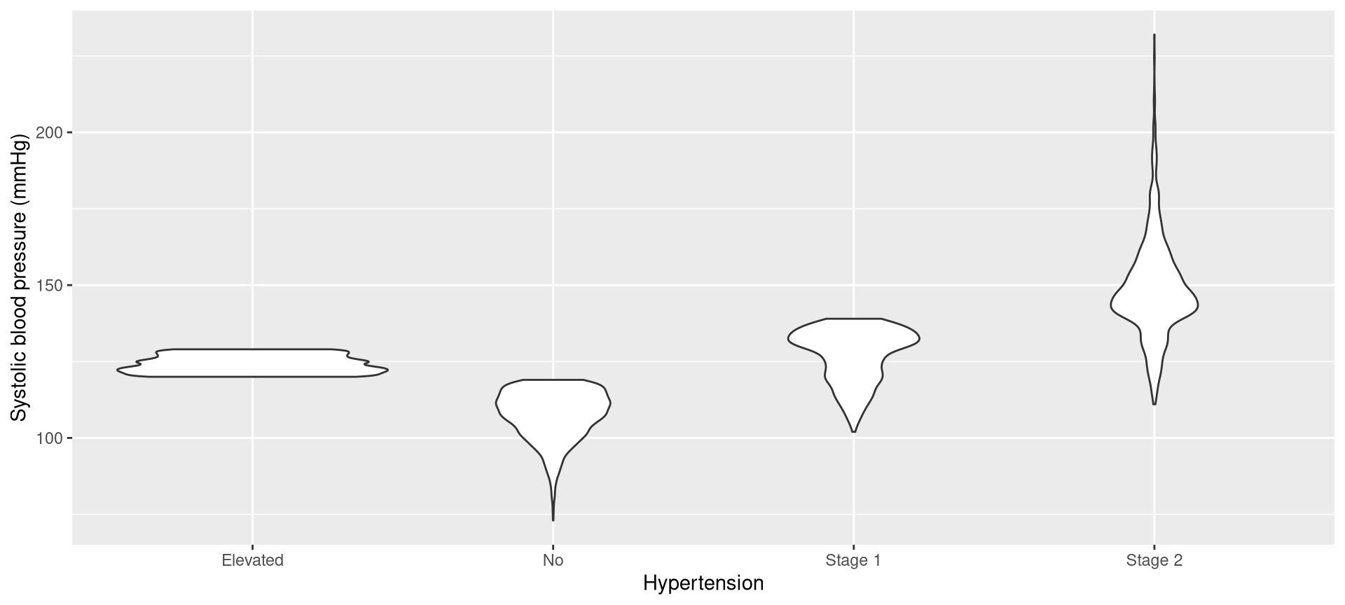
Hypertension

table(nhanes$hypertension)
#|  
#|  Elevated       No  Stage 1  Stage 2 
#|       841     2657     1409     1216

Hypertension

class(nhanes$hypertension)
#|  [1] "character"

• groups in character variables are always presented in alphabetical order

Hypertension

• to specify the desired order of the groups, convert the object type to a factor:

nhanes$ht<-factor(nhanes$hypertension,
                  levels=c('No','Elevated','Stage 1','Stage 2'))

• there are two arguments to factor() here:
  • nhanes$hypertension: the original variable
  • c('No',...): the groups listed in the desired order
• it is not necessary to type the argument name

Hypertension

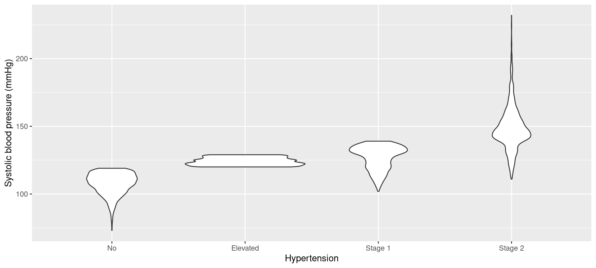
Hypertension

table(nhanes$ht)
#|  
#|        No Elevated  Stage 1  Stage 2 
#|      2657      841     1409     1216

Factors

class(nhanes$ht)
#|  [1] "factor"
is.vector(nhanes$ht)
#|  [1] FALSE
head(nhanes$ht)
#|  [1] Stage 2 Stage 1 No      <NA>    <NA>    No     
#|  Levels: No Elevated Stage 1 Stage 2

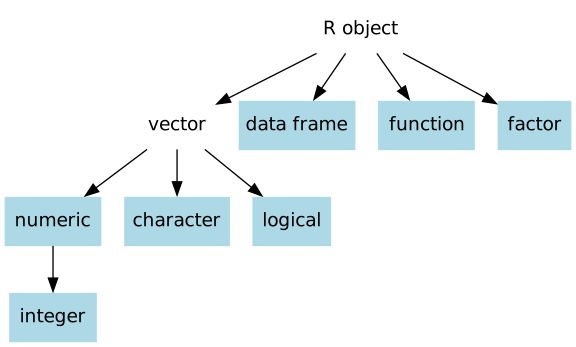
Factors

Free text versus multiple choice

• free text: Please tell me, in as few or as many words as you like, how much or how little you liked this ice cream.
• multiple choice: How much did you like this ice cream? Select just one of the following.
  • I hated it
    
  • I disliked it
  • It was OK
  • I liked it
  • I loved it

Character versus factor

• free text → character
• multiple choice → factor

Character versus factor

	best for these data	possible values	groups can be ordered
character	free text	many	no
factor	multiple choice	limited	yes

Factor levels

levels(nhanes$ht)
#|  [1] "No"       "Elevated" "Stage 1"  "Stage 2"

• factor groups are known as levels

Factors in regression models

• if a factor is used as an x variable, the first group is the reference
• in logistic regression, if a factor is used as a y variable, the second group is used as the “yes” outcome

Exercise 1

Exercise 1

1. At the top of a new script, include code for importing the data. Run your code.

2. table() the cholesterol variable (cholesterol). Which group is listed first? Check the object type. What is the object type?

Exercise 1

3. Use factor() to re-order the groups in cholesterol so that they are in the following order: Desirable, Borderline high, and High. You can create a new variable (such as cholesterol_factor) or overwrite the existing cholesterol variable. Check your work. Verify that the groups are listed in the desired order in table().

Labeling groups

Country of birth

table(nhanes$dmdborn4,useNA='always')
#|  
#|     1    2 <NA> 
#|  6519 1617   17

Country of birth

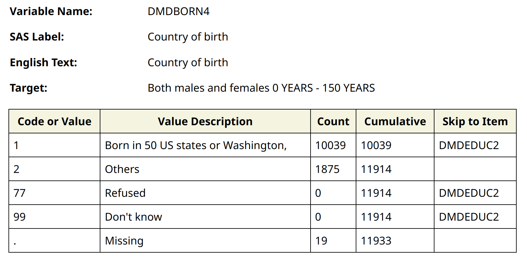
• from NHANES:

Country of birth

• to label the groups, convert the variable to a factor and include the labels argument:

nhanes$country<-factor(nhanes$dmdborn4,
                       levels=c(1,2),
                       labels=c('USA','Other'))

• the order of the groups in levels and labels must match

table(nhanes$country,useNA='always')
#|  
#|    USA Other  <NA> 
#|   6519  1617    17

Country of birth

• alternatively, use the base_match() function in baseverse:

nhanes$country<-base_match(nhanes$dmdborn4,'USA'=1,'Other'=2)

• the second argument lists the value–label mappings in a 'label'=value format
• base_match() will honor the order of the groups

Country of birth

table(nhanes$country,useNA='always')
#|  
#|    USA Other  <NA> 
#|   6519  1617    17

• base_match() orders the groups in the order specified in the second argument

Country of birth

• to check the work, use table():

table(nhanes$dmdborn4,useNA='always')
#|  
#|     1    2 <NA> 
#|  6519 1617   17
table(nhanes$country,useNA='always')
#|  
#|    USA Other  <NA> 
#|   6519  1617    17

Education

table(nhanes$dmdeduc2,useNA='always')
#|  
#|     1    2    3    4    5    9 <NA> 
#|   373  666 1749 2370 2625   11  359

Education

• from NHANES:

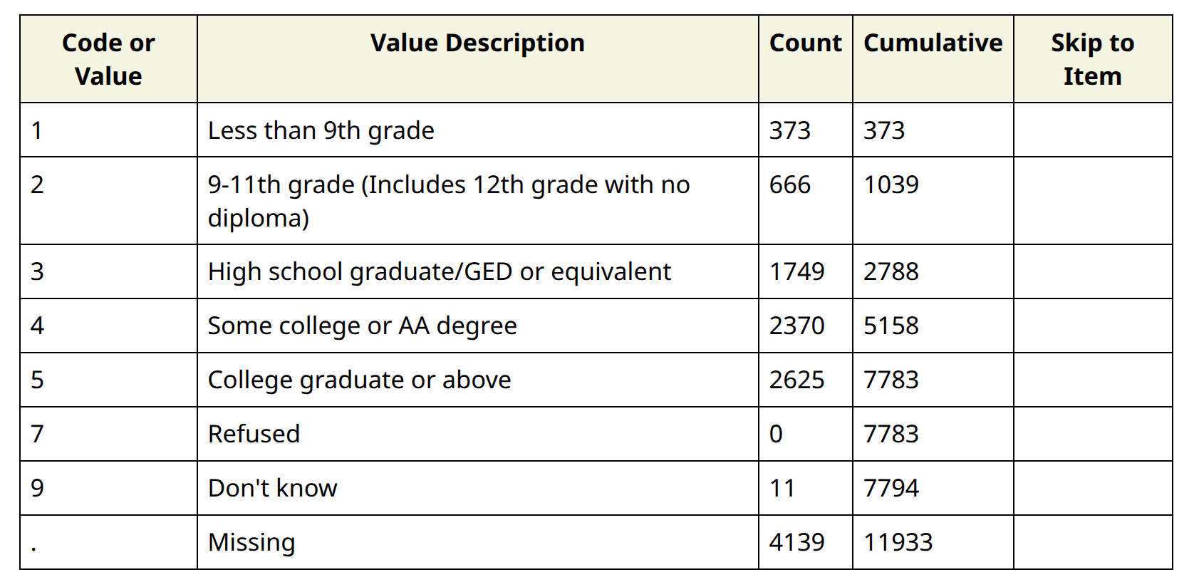
Education

• to collapse groups and label them, use base_match() and list the groups more than once:

nhanes$education4<-base_match(nhanes$dmdeduc2,
                              'No high-school degree'=1,
                              'No high-school degree'=2,
                              'High-school degree'=3,
                              'Some college'=4,
                              'College degree'=5)

Education

• to check the work, use table():

table(nhanes$dmdeduc2,useNA='always')
#|  
#|     1    2    3    4    5    9 <NA> 
#|   373  666 1749 2370 2625   11  359
table(nhanes$education4,useNA='always')
#|  
#|  No high-school degree    High-school degree          Some college 
#|                   1039                  1749                  2370 
#|         College degree                  <NA> 
#|                   2625                   370

Exercise 2

Exercise 2

1. Add code for loading baseverse to the top of your script. Run your code.

Exercise 2

2. Use base_match() to create a labeled version of the original gender variable (riagendr). Name the new variable gender_base. Values of 1 represent males and values of 2 represent females. List the male group first. Check your work. Verify that the groups are listed in the desired order in table().

I don’t have a personal preference regarding whether male or female is listed first! I’m only having you list male first to prove that base_match() will provide a non-alphabetical order, if you request it.

Exercise 2

3. Use base_match() to create a labeled version of race/ethnicity (ridreth3). You can call this variable race or race_ethnicity or whatever else makes sense to you. You may list the groups in whatever order you like. The NHANES documentation for ridreth3 is available here. Check your work. Verify that the groups are listed in the desired order in table().

Exercise 2

4. Add code for loading dplyr to the top of your script. Run your code.

5. Use case_match(), from dplyr, to create another labeled version of the original gender variable (riagendr). Name the new variable gender_dplyr. Again, list the male group first. case_match() works similarly to base_match(), except the value–label mappings should be listed in a value ~ 'label' format.

It is more common to implement case_match() in a different way, using something called piping, but that is outside the intended scope of this series.

Exercise 2

6. table() the gender_base variable. Check the class of the variable. What do you notice about the order of the groups and the object class?

7. table() the gender_dplyr variable. Check the class of the variable. What do you notice about the order of the groups and the object class?

Categorizing continuous variables

Total cholesterol

range(nhanes$lbxtc,na.rm=TRUE)
#|  [1]  62 438

• lbxtc < 200 mg/dL → desirable
• 200 ≤ lbxtc < 240 mg/dL → borderline high
• lbxtc ≥ 240 mg/dL → high

Total cholesterol

• to categorize total cholesterol, use base_when():

nhanes$cholesterol<-base_when(
   'Desirable' = (nhanes$lbxtc<200),
   'Borderline high' = (nhanes$lbxtc>=200)&(nhanes$lbxtc<240),
   'High' = (nhanes$lbxtc>=240)
)

• each argument of base_when() is a rule–label mapping in a label=rule format
• base_when() will honor the order of the groups

The nhanes_l.csv data file already includes a cholesterol variable. I’m overwriting it here.

Total cholesterol

• to omit dollar-sign notation, use with():

nhanes$cholesterol<-with(nhanes,base_when(
   'Desirable' = (lbxtc<200),
   'Borderline high' = (lbxtc>=200)&(lbxtc<240),
   'High' = (lbxtc>=240)
))

Total cholesterol

• to check the work, use sum() and table():

sum(nhanes$lbxtc<200,na.rm=TRUE)
#|  [1] 3695
sum((nhanes$lbxtc>=200)&(nhanes$lbxtc<240),na.rm=TRUE)
#|  [1] 1397
sum(nhanes$lbxtc>=240,na.rm=TRUE)
#|  [1] 625
table(nhanes$cholesterol,useNA='always')
#|  
#|        Desirable Borderline high            High            <NA> 
#|             3695            1397             625            2436

Exercise 3

Exercise 3

1. Use base_when() to define a variable for age group, with the following groups: 18–34, 35–54, and ≥ 55. The original age variable is ridageyr. Name the variable age3_base. Use the following labels: Youngest, Middle, and Oldest, and list the groups in that order. Check your work. Verify that the groups are listed in the desired order in table().

I wouldn’t actually use these group names in practice. I’m suggesting them here just so you can verify a non-alphabetical order of the groups later.

Exercise 3

2. Copy and paste code from Session 6 for defining minutes of vigorous physical activity, with the NA values properly encoded. Now, use base_when() to define a categorical physical-activity variable with the following groups: less than 60 minutes, 60 minutes to less than 120 minutes, and 120 minutes or more. List the groups in order from fewer minutes to more minutes. Check your work. Verify that the groups are listed in the desired order in table().

Exercise 3

3. Use case_when(), from the dplyr, to create another variable for age group, with the following groups: 18–34, 35–54, and ≥ 55. The original age variable is ridageyr. Name the variable age3_dplyr. Use the following labels: Youngest, Middle, and Oldest, and list the groups in that order. case_when() works similarly to base_when(), except the rule–label mappings should be listed in a rule ~ 'label' format.

It is more common to implement case_when() in a different way, using something called piping, but that is outside the intended scope of this series.

Exercise 3

4. table() the age3_base variable. Check the class of the variable. What do you notice about the order of the groups and the object class?

5. table() the age3_dplyr variable. Check the class of the variable. What do you notice about the order of the groups and the object class?

Beyond today

Other workshops I teach

• something on Quarto: possibly in Winter quarter
  • Quarto is a very popular tool for generating reports, slide decks (such as this one), and websites
• Data Manipulation in R: in Winter or Spring quarter
  • includes an introduction to dplyr and the tidyverse way of doing things
  • includes base-R and dplyr solutions
  • covers techniques for merging data and reshaping data

Other topics you might pursue

• mapping and GIS
• interactive data visualizations
• Shiny: a tool for creative interactive websites

Other topics you might pursue

• multiple imputation and other approaches for dealing with missing data
• packages for survey analysis

Other topics you might pursue

• bracket notation (indexing): a base-R technique for subsetting data and manipulating data
• repetition: for() loops, the apply functions, and other tools
• writing your own functions
• regular expressions: for searching through text and replacing text
• packages for parallel computing