nhanes<-read.csv('~/Downloads/data/nhanes/l/nhanes_l.csv')Homework 4
At the top of a new script, include code for importing the
nhanes_l.csvdata file. Run that code.TipSolutionCreate a box plot of the typical number of sleep hours (
sld012) versus occupation status (ocd150). Label the y axis and optionally remove the label for the x axis. The occupation variable codes groups using numbers; a description is available here. We’ll talk in Session 7 about how to “label” categorical variables that use numeric codes.You may notice that
9codes people who indicated that they don’t know how much sleep they typically get. We’ll talk in Session 6 about how to properly encode missing values.TipSolutionboxplot(nhanes$sld012~nhanes$ocd150,ylab='Hours of sleep',xlab='')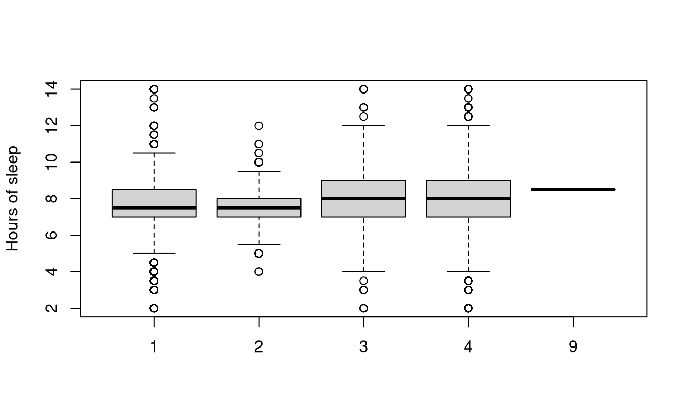
Create a box plot of the typical number of sleep hours (
sld012) versus gender (gender). Label the y axis and optionally remove the label for the x axis.TipSolutionboxplot(nhanes$sld012~nhanes$gender,ylab='Hours of sleep',xlab='')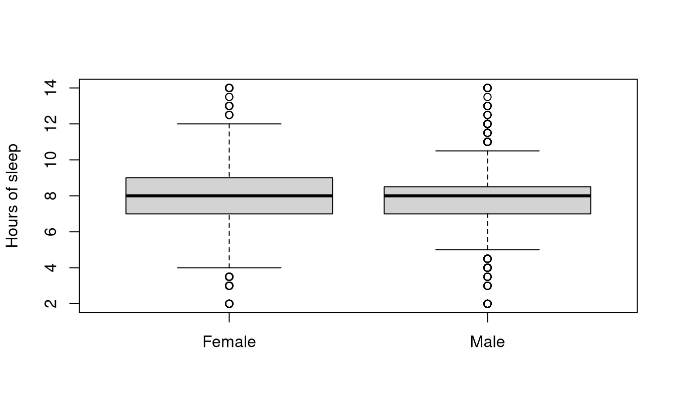
Conduct a t-test for the association between the typical number of sleep hours (
sld012) and gender (gender).TipSolutiont.test(nhanes$sld012~nhanes$gender) #| #| Welch Two Sample t-test #| #| data: nhanes$sld012 by nhanes$gender #| t = 4.8356, df = 7638.6, p-value = 1.353e-06 #| alternative hypothesis: true difference in means between group Female and group Male is not equal to 0 #| 95 percent confidence interval: #| 0.1044477 0.2468641 #| sample estimates: #| mean in group Female mean in group Male #| 7.820103 7.644448Create a contingency table for country of birth (
dmdborn4) and asthma (asthma), with country of birth placed along the rows.The country variable codes groups using numbers; a description is available here. We’ll talk in Session 7 about how to “label” categorical variables that use numeric codes.
TipSolutiontable(nhanes$dmdborn4,nhanes$asthma) #| #| History of asthma No #| 1 1286 5226 #| 2 198 1417Find the row-wise percents.
TipSolutionprop.table(table(nhanes$dmdborn4,nhanes$asthma),1)*100 #| #| History of asthma No #| 1 19.74816 80.25184 #| 2 12.26006 87.73994Conduct a chi-squared test for the association between the two variables.
TipSolutionchisq.test(table(nhanes$dmdborn4,nhanes$asthma)) #| #| Pearson's Chi-squared test with Yates' continuity correction #| #| data: table(nhanes$dmdborn4, nhanes$asthma) #| X-squared = 48.114, df = 1, p-value = 4.022e-12