Session 3: How can I perform univariate analysis?

A Slower Introduction to R

Yea-Hung Chen, PhD, MS

UCSF Library

Thursday, October 23, 2025

Arguments

The NA mean

• from last week:

mean(nhanes$bpxodi1)
#|  [1] NA
class(nhanes$bpxodi1)
#|  [1] "integer"
head(nhanes$bpxodi1)
#|  [1] 98 84 79 NA NA 72

The help pages

• to access the help page for a function, use the help() function:

> help(sqrt)

• or, equivalently, use ?:

> ?sqrt

Live demonstration

Function arguments in sqrt()

• you can optionally type x= when you use sqrt():

sqrt(x=81)
#|  [1] 9

• or, you can continue to omit it:

sqrt(81)
#|  [1] 9

• x is known as an argument

What are function arguments?

• you may think of arguments as being like options or settings
• using another cooking analogy, suppose that baking is a function
  • we can think of the temperature setting on the oven as an argument to the function
  • what’s another possible argument to baking?

What are function arguments?

sqrt(x=81)
#|  [1] 9

• 81 is the argument value
• x is the argument name

Function arguments in mean()

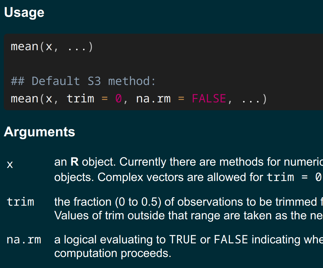
• notice the commas and the default values

Function arguments in mean()

• the na.rm argument is:

a logical evaluating to TRUE or FALSE indicating whether NA values should be stripped before the computation proceeds.

• the Usage section (previous slide) shows that the default value for na.rm is FALSE, suggesting that NA values will not be “stripped”

The missing mean

mean(nhanes$bpxodi1,na.rm=TRUE)
#|  [1] 74.97469

🎉🎉🎉

The missing mean

mean(nhanes$bpxodi1,na.rm=TRUE)
#|  [1] 74.97469

• notice that I’ve used a comma to separate the two arguments
• TRUE must be in all caps
• na.rm=TRUE does not delete missing values from your data
• all it does is make mean() ignore missing values

na.rm

Caution

The na.rm argument does not exist in every R function!

• most of the functions in the next section have an na.rm argument
• but, for example, the function for linear regression, lm(), does not have an na.rm argument

When should I include argument names?

sqrt(x=81)
#|  [1] 9
sqrt(81)
#|  [1] 9

• if there is just one argument, the argument name is optional

When should I include argument names?

mean(nhanes$bpxodi1,na.rm=TRUE)
#|  [1] 74.97469

• if there is more than one argument, you should include argument names if:
  • you skip an argument
  • or, write the arguments out of order

When should I include argument names?

sd(nhanes$bpxodi1,TRUE)
#|  [1] 11.41659
sd(nhanes$bpxodi1,na.rm=TRUE)
#|  [1] 11.41659

• regardless of the considerations on the prior slides, including argument names can improve the readability of your code

Writing across multiple lines

• when writing across multiple lines, type the comma before the line break:

mean(nhanes$bpxodi1,
     na.rm=TRUE)

Exercise 1

Exercise 1

1. Open the help page for the quantile() function, which you’ll use in Exercise 2 to find percentiles of continuous variables.
2. What is the name of the second argument?
3. Does the function support the na.rm argument?

Summarizing continuous variables

What is a continuous variable?

• continuous variable = a variable that has numeric values
• examples:
  • age
  • height
  • systolic blood pressure

Means, standard deviations, and variances

mean(nhanes$bpxodi1,na.rm=TRUE)
#|  [1] 74.97469
sd(nhanes$bpxodi1,na.rm=TRUE)
#|  [1] 11.41659
var(nhanes$bpxodi1,na.rm=TRUE)
#|  [1] 130.3386

Percentiles

median(nhanes$bpxodi1,na.rm=TRUE)
#|  [1] 74
quantile(nhanes$bpxodi1,probs=0.5,na.rm=TRUE)
#|  50% 
#|   74
quantile(nhanes$bpxodi1,0.5,na.rm=TRUE)
#|  50% 
#|   74

Percentiles

quantile(nhanes$bpxodi1,0.25,na.rm=TRUE)
#|  25% 
#|   67
quantile(nhanes$bpxodi1,0.75,na.rm=TRUE)
#|  75% 
#|   82

Percentiles

> quantile(nhanes$bpxodi1,c(0.25,0.5,0.75),na.rm=TRUE)
25% 50% 75% 
 67  74  82 

• in the second argument, we’ve used the c() function to create a vector containing 3 values

Minimum and maximum values

min(nhanes$bpxodi1,na.rm=TRUE)
#|  [1] 36
max(nhanes$bpxodi1,na.rm=TRUE)
#|  [1] 142
range(nhanes$bpxodi1,na.rm=TRUE)
#|  [1]  36 142

summary()

summary(nhanes$bpxodi1)
#|     Min. 1st Qu.  Median    Mean 3rd Qu.    Max.    NA's 
#|    36.00   67.00   74.00   74.97   82.00  142.00    2030

Histograms

hist(nhanes$bpxodi1)

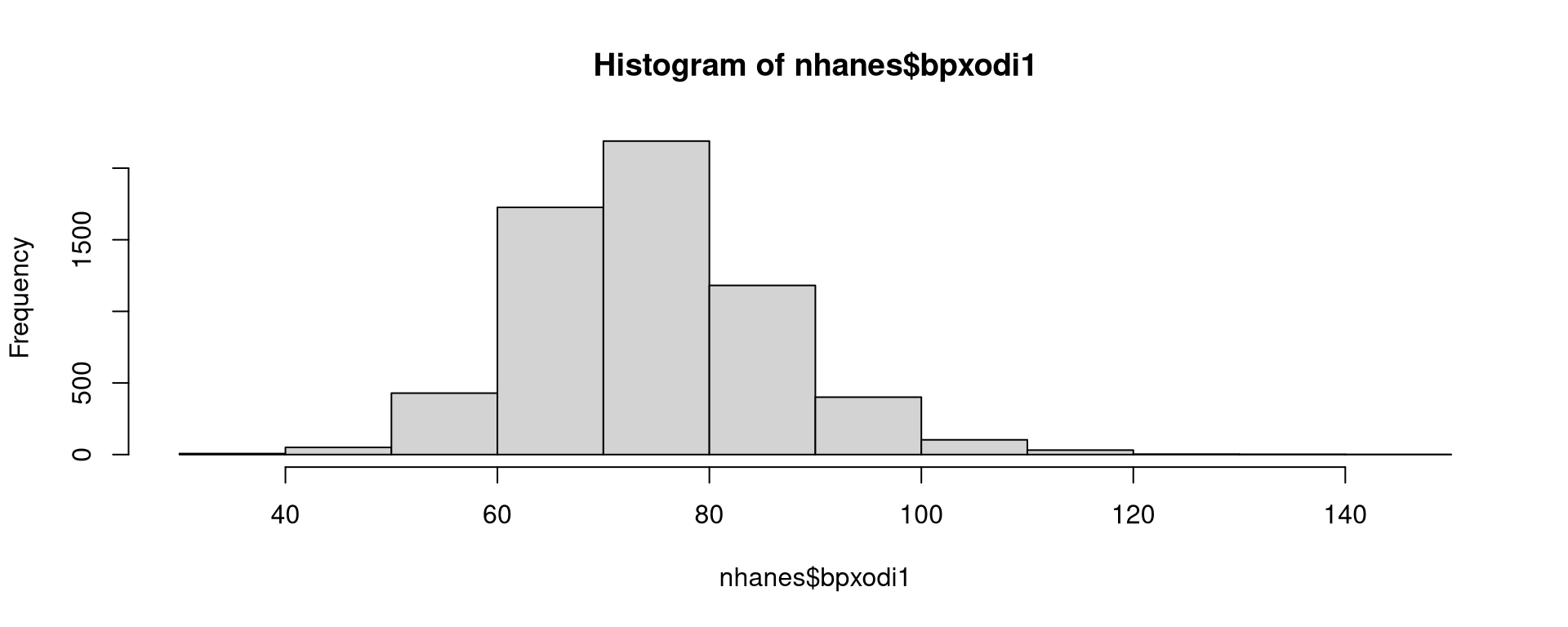
Histogram titles and labels

• main: the title at the top
• xlab: the label on the x axis

Histograms titles and labels

hist(nhanes$bpxodi1,main='',xlab='Diastolic blood pressure (mmHg)')

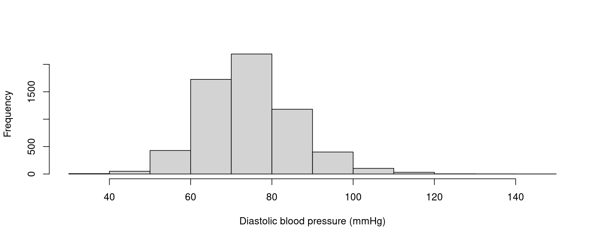
Histogram bars

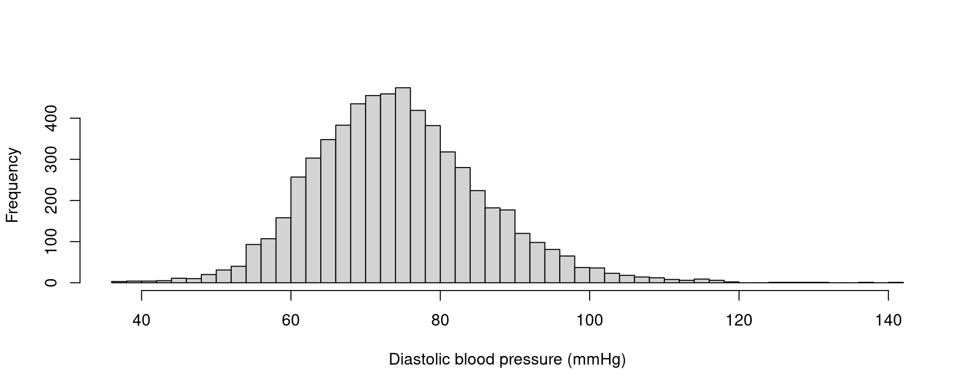
• to set the number of bars in the histogram, use the breaks argument

hist(nhanes$bpxodi1,main='',xlab='Diastolic blood pressure (mmHg)',breaks=50)

When you use breaks in this way, you won’t always get exactly the number of bars you requested.

Histograms bars

hist(nhanes$bpxodi1,main='',xlab='Diastolic blood pressure (mmHg)',breaks=50)

Quotes in function arguments

Tip

If a function argument needs to be in quotes, you can use single quotes or double quotes.

hist(nhanes$bpxodi1,main='',xlab="Diastolic blood pressure (mmHg)",breaks=50)

• if you start with a single quote, you must end with a single quote
• and, if you start with a double quote, you must end with a double quote

Exercise 2

Exercise 2

Across the exercises today, you’ll build an R script that will import the NHANES data and perform some univariate analysis. You’ll also practice going back and forth between the console and your script.

1. At the top of a new script, include code for importing the data. Hopefully, you already copied and pasted code for doing this from last week. If you didn’t, re-obtain the code by using RStudio’s import tool. Add a comment above that code. Run that code.

Exercise 2

2. In the console or the script, write code for displaying a histogram of fasting glucose (lbxglu). Now do this again, specifying that you want to use 60 bins. Feel free to try other numbers of bins.

3. A common threshold for a health level of fasting glucose is 100 mg/dL. In the console or the script, add a red vertical line to your histogram at that threshold: abline(v=100,col='red').

Exercise 2

4. In the script, type code for finding the mean level of fasting glucose. Add a comment above that code. Run that code.

5. In the script, type code for finding the 25th, 50th, and 75th percentiles of fasting glucose. Add a comment above that code. Run that code.

Confidence intervals for population means

Confidence interval for mean diastolic blood pressure

• what is a 95% confidence interval for the mean diastolic blood pressure in the US adult population?

t.test(nhanes$bpxodi1)
#|  
#|      One Sample t-test
#|  
#|  data:  nhanes$bpxodi1
#|  t = 513.88, df = 6122, p-value < 2.2e-16
#|  alternative hypothesis: true mean is not equal to 0
#|  95 percent confidence interval:
#|   74.68867 75.26070
#|  sample estimates:
#|  mean of x 
#|   74.97469

Function values

• t.test() prints a summary report
• it is possible to extract specific values

Function values

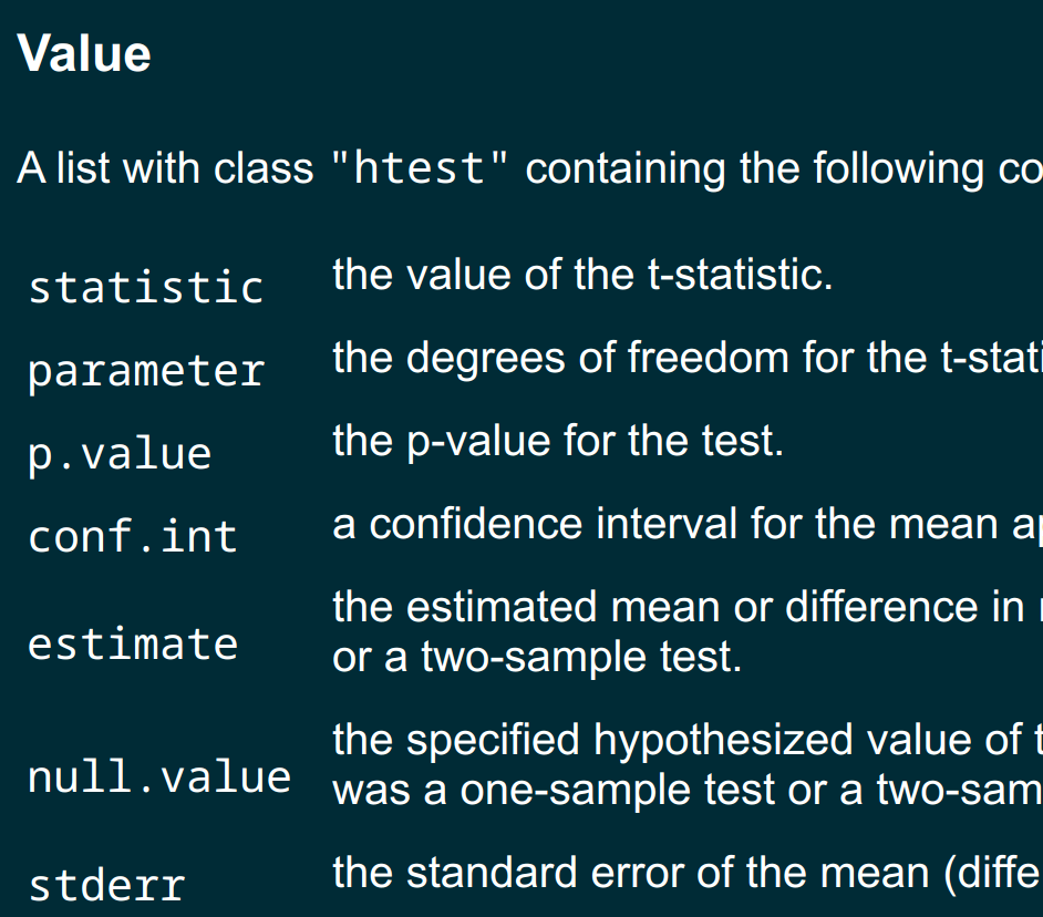
Function values

diastolic_ci<-t.test(nhanes$bpxodi1)
names(diastolic_ci)
#|   [1] "statistic"   "parameter"   "p.value"     "conf.int"    "estimate"   
#|   [6] "null.value"  "stderr"      "alternative" "method"      "data.name"

Extracting function values

diastolic_ci$estimate
#|  mean of x 
#|   74.97469
diastolic_ci$conf.int
#|  [1] 74.68867 75.26070
#|  attr(,"conf.level")
#|  [1] 0.95

Summarizing categorical variables

What is a categorical variable?

• categorical variable = a variable that has groups
• examples:
  • age group
  • level of educational attainment
  • exposure (yes or no)
  • disease (yes or no)
• variables with two groups are known as dichotomous variables

Hypertension

class(nhanes$hypertension)
#|  [1] "character"
head(nhanes$hypertension)
#|  [1] "Stage 2" "Stage 1" "No"      NA        NA        "No"

Counts

table(nhanes$hypertension)
#|  
#|  Elevated       No  Stage 1  Stage 2 
#|       841     2657     1409     1216

Missing values?

• what about the missing values?

The help page for table()

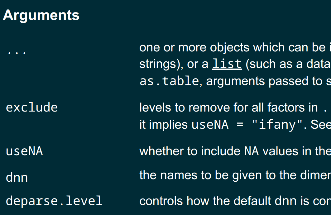
The help page for table()

• the useNA argument can be used to control:

whether to include NA values in the table

Counts

table(nhanes$hypertension,useNA='always')
#|  
#|  Elevated       No  Stage 1  Stage 2     <NA> 
#|       841     2657     1409     1216     2030
table(nhanes$hypertension,useNA='ifany')
#|  
#|  Elevated       No  Stage 1  Stage 2     <NA> 
#|       841     2657     1409     1216     2030

Percents

prop.table(table(nhanes$hypertension,useNA='always'))
#|  
#|   Elevated        No   Stage 1   Stage 2      <NA> 
#|  0.1031522 0.3258923 0.1728198 0.1491476 0.2489881

• notice that you must put table() inside of prop.table()

Percents

• without the NA included:

prop.table(table(nhanes$hypertension))
#|  
#|   Elevated        No   Stage 1   Stage 2 
#|  0.1373510 0.4339376 0.2301160 0.1985955

Percents

• on a percent scale:

prop.table(table(nhanes$hypertension,useNA='always'))*100
#|  
#|  Elevated       No  Stage 1  Stage 2     <NA> 
#|  10.31522 32.58923 17.28198 14.91476 24.89881

Percents

prop.table(table(nhanes$hypertension))*100
#|  
#|  Elevated       No  Stage 1  Stage 2 
#|  13.73510 43.39376 23.01160 19.85955

Exercise 3

Exercise 3

1. In the script from Exercise 2, write code for obtaining the percent of adults who have a history of smoking (smoking). Add a comment above that code. Run that code.

2. In the script, write code for obtaining the percent of adults who have a history of asthma (asthma). Add a comment above that code. Run that code.

Exercise 3

3. Select all of the text and code in your script. You can optionally use a keyboard shortcut: ctrl + A on Windows machines or cmd + A on Mac machines. Run the code, and verify that your computer reproduced all of the work.