Session 2: How can I import data?

A Slower Introduction to R

Yea-Hung Chen, PhD, MS

UCSF Library

Thursday, October 16, 2025

Scripts

Yet another cooking analogy

sometimes I can’t quite remember what I did in the kitchen
what is a possible solution?

Yet another cooking analogy

using the console is like winging it in the kitchen

What are scripts?

scripts = documents that you can use to store code
continuing the analogy, scripts are like recipes

Why should I use scripts?

scripts are a way for you to save and revisit your work, much the same way a recipe would allow you to cook the same dish again
scripts help promote transparency and reproducibility

Scripts in RStudio

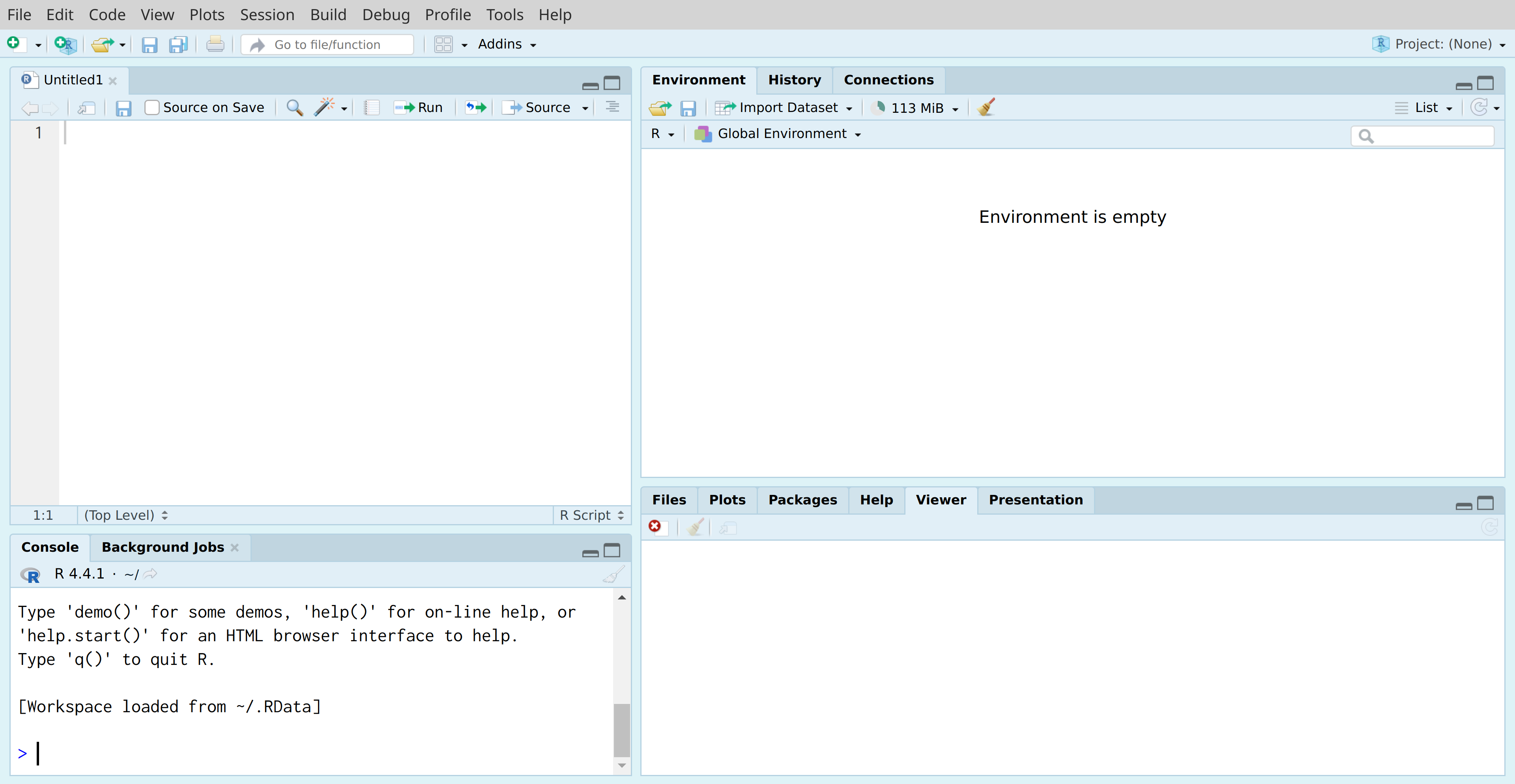
Running scripts

you can send code from scripts to your computer
this process is known as running the code, and will result in the code and output showing up in the console

Live demonstration

🤸

Running code

Select the code.
Run the code, using either the Run icon at the top of the pane or the keyboard shortcut (ctrl + enter on Windows or cmd + return on Mac).

One line for each statement

Caution

Each statement (“sentence”) of code should be on its own line.

for example, you cannot do this:

sqrt(81) pi^2

you should, instead, do this:

sqrt(81) 
pi^2

Long statements

if you wish, you can write a statement of code that spans more than one line:

(0.25*0.4)/
  (0.25*0.4+(1-0.9)*(1-0.4))

Long statements

Caution

If you are writing a sentence of code that spans more than one line, always place mathematical operators before the line break rather than after the line break.

Long statements

this will work as intended:

5*12+
  2

this will not work as intended and will not result in an error:

5*12
  +2

why?

Comments

you can include human-language comments in scripts
comments serve as notes for yourself and for your collaborators

Adding comments

to include comments in scripts, begin the line with the pound sign

# calculate positive predictive value when prevalence is 0.4
(0.25*0.4)/(0.25*0.4+(1-0.9)*(1-0.4))

# calculate positive predictive value when prevalence is 0.3
(0.25*0.3)/(0.25*0.3+(1-0.9)*(1-0.3))

Live demonstration

🤸

Saving scripts

Click the save icon at the top of the pane or, equivalently, select File > Save.
Select a folder if you don’t want to save the file to the folder being suggested to you.
Pick a filename, making sure to add .r or .R to the end.

Exercise 1

Check whether or not a blank script is already open (the tab might be labeled Untitled1). If not, open a new script by selecting File > New File > R Script.
A common cutoff for a borderline high LDL cholesterol level is 130 mg/dL. In the first line of your script, type code that stores the value of 130 as ldl_borderline, using object assignment.

Exercise 1

A common cutoff for a high LDL cholesterol level is 160 mg/dL.In the second line, type code that stores the value of 160 as ldl_high, using object assignment.
Add a comment above each object assignment that describes the object assignment. For readability, include a blank line between the first object assignment and the second comment.

Exercise 1

Select and run your code.
In the console, check to see that ldl_borderline and ldl_high were properly defined (type each object name and press the enter or return key on your keyboard).
Save the script, picking some filename that makes sense to you (such as session_2.r). Make sure to add .r or .R at the end. You might first create a folder on your computer for this workshop series.

Suggested workflow

Slide formatting

to facilitate copying-and-pasting, throughout the remainder of the workshop series, I will omit the prompt
for example:

(0.25*0.4)/(0.25*0.4+(1-0.9)*(1-0.4))
#|  [1] 0.625

this does not necessarily mean that you should use a script over a console
what do I suggest?

Should I use the script or the console?

Tip

Go back and forth between the script and the console.

there are two ways to do this:
1. try things out in the console and then copy and paste code into your script
2. type in the script, run your code, and examine the output in the console

Should I use the script or the console?

as you get more experienced with R, you will probably do most of your typing in scripts

How can I save my work?

Tip

Use scripts as a way to save work!

I discourage you from trying to save work by relying on objects
instead, lean on scripts

How should I structure my scripts?

Tip

Your scripts should have a sequence.

as with the recipes analogy, the idea is that the script should serve as a record of your work, and have a general top-to-bottom flow

How should I keep my scripts clean?

Tip

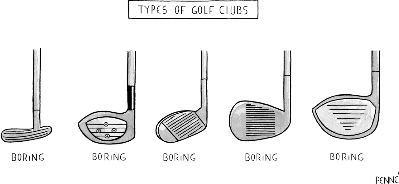
Only include code and comments.

do not include un-commented human-language text!
do not include output!

How can I facilitate readability?

Tip

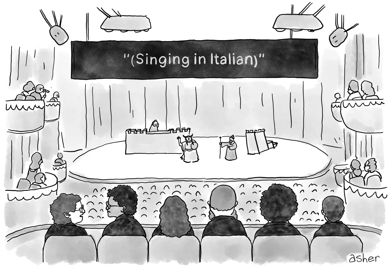
Write comments.

How can I facilitate readability?

I like to write short but frequent comments
I like to begin every comment with a verb

# import data
nhanes<-read.csv('~/Downloads/data/acs/2019/psam_p06.csv.gz')

# rename variables
names(nhanes)<-tolower(names(nhanes))

# subset to individuals 18-65 years of age
nhanes<-subset(nhanes,agep>=18&agep<=65)

How can I facilitate readability?

“I kinda thought the subtitles would be more helpful.”

What if my script is really long?

Tip

Consider using more than one script.

the scripts should have a natural sequence from one to another, such as:
1. import and prepare data.r
2. analyze data.r

How can I write good code and avoid mistakes?

Tip

Continually revisit your scripts!

think of a script as being like a work-in-progress manuscript
be willing to continually edit it

Importing data

NHANES

the National Health and Nutrition Examination Survey (NHANES) is a large, CDC survey of American health:

The National Health and Nutrition Examination Survey (NHANES) collects data about the health of adults and children in the United States. We also collect data about what participants eat, drink, and take as supplements to determine how many nutrients are in their diet.

NHANES

nhanes_l.csv, available on the CLE, contains data from the 2021–2023 implementation of NHANES
I created the file by combining (merging) several CDC data files, from across several dimensions
I restricted the data to individuals 18 years of age or older
I added a handful of variables, using existing variables
the original data, and data descriptions, are available here

Importing the data

as mentioned in the orientation, there are often many ways to do something in R
I’m going to show you how to use RStudio’s drop-down menu to import the data
as a preview, this process will result in object assignment

Live demonstration

🤸

Importing the data

in our quick demonstration we changed two parts of the pop-up window:
- Name: the name from the resulting object assignment (using the jar analogy, this is the label you put on the jar)
- Heading: an option that indicates whether or not variables are included as the first line of the data file

The corresponding code

the import tool will print the corresponding R code in the console
that code involves object assignment

The corresponding code

Tip

Examine the code to begin to understand it.

The corresponding code

Tip

Copy and paste the corresponding code to a script so you can later reproduce the import without having to rely on the import tool.

it is not necessary to copy the View() portion of the code

The view tab

by default, the import tool will automatically show the data in a new tab in the Source pane
you can close the tab if you want (the object itself will not be removed)
you can always open the view tab again by using View()

The view tab

Tip

Examine the data carefully after importing a data file for the first time.

check that variable names are there (if they should be there)
scroll through to check to see that columns are lined up properly

Other ways to explore the data

names(): for all the variable names
head(): for the first few rows
tail(): for the last few rows
str(): for a glimpse of the data that shows variable names, object classes (more about this later), and the first few values

Other ways to explore the data

dim(): for the number of rows and the number of columns, in that order
nrow(): for the number of rows
ncol(): for the number of columns

Other ways to explore the data

dim(nhanes)
#|  [1] 8153  195
nrow(nhanes)
#|  [1] 8153
ncol(nhanes)
#|  [1] 195

Exercise 2

Download the data from the CLE, by clicking on the link, and then browsing for a folder on your computer where you would like to save the file. If the data opens in your browser instead, go back to the CLE page and instead right-click on the link (or control-click or two-finger click), and select save.
Use RStudio’s drop-down menu to import the data: File > Import Dataset > From Text (base). Please make sure to select the base option.

Exercise 2

In the pop-up window, select Yes under the Heading option.
Confirm that the data look OK in the preview section at the bottom right. If so, select the Import button.

Exercise 2

Confirm that the data look OK in the viewer that pops up (in the Source pane). You can optionally close the tab when you’re done.
Copy and paste the code for importing the data into your script.
Use head() to view the first few rows of the data.

Dollar-sign notation

An error message

the mean() function will find the mean of a set of numbers
there is a variable in the data called ridageyr, which stores ages in years
we might be inclined to try this:

mean(ridageyr)
#|  Error:
#|  ! object 'ridageyr' not found

why do we get an error message?

An error message

we get an error message because R allows multiple data sets to be available at a time
so, any time we refer to a variable we also have to refer to the data set

Dollar-sign notation

mean(nhanes$ridageyr)
#|  [1] 52.14436

mean(): a function for finding the arithmetic mean
nhanes: the label we gave for our data when we imported it
$: indicates that ridageyr is a column in nhanes
ridageyr: the variable name

Exercise 3

The head() and tail() functions, mentioned earlier, can be used not only to preview data but also to preview variables within data. Use these functions to view the first few, and the last few, values of the gender variable.
The range() function will show the range of a variable (this is, the minimum and maximum values). Use range() to find the age range of individuals in the NHANES data (the age variable is ridageyr).

Object classes

Another error message

mean(nhanes$gender)
#|  Warning in mean.default(nhanes$gender): argument is not numeric or logical:
#|  returning NA
#|  [1] NA

there is a variable in the NHANES data called gender
we are using dollar-sign notation
so, why does this result in an error?

Another error message

we got an error message because gender does not include numbers:

head(nhanes$gender)
#|  [1] "Male"   "Male"   "Female" "Male"   "Female" "Male"

Object classes

a more general way to check is to use the class() function:

class(nhanes$gender)
#|  [1] "character"

Object classes

the class() function reports the object type
R has many different object types
the formal term for object types is object classes
using the jar analogy, you can think of object classes as being like the different types of ingredients you might have inside of jars

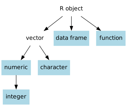
A taxonomy of object classes

Vectors

class(nhanes$ridageyr)
#|  [1] "integer"
is.vector(nhanes$ridageyr)
#|  [1] TRUE
class(nhanes$gender)
#|  [1] "character"
is.vector(nhanes$gender)
#|  [1] TRUE

integer and character objects are examples of vectors

Numeric objects

is.numeric(nhanes$ridageyr)
#|  [1] TRUE
is.integer(nhanes$ridageyr)
#|  [1] TRUE
is.numeric(22.52)
#|  [1] TRUE
is.integer(22.52)
#|  [1] FALSE

integer objects are themselves examples of numeric objects, but not all numeric objects are integers

A taxonomy of object classes

Data frames and functions

class(nhanes)
#|  [1] "data.frame"
class(mean)
#|  [1] "function"

A taxonomy of object classes

Object classes

mostly I just want you to begin to be aware of all of this because classes will determine what you can and cannot do with objects, as illustrated in the first example

Exercise 4

The bpxodi1 variable stores measurements of diastolic blood pressure. Try to find the mean of this variable. You should see a value of NA.
Now check the class of this variable. You should see that the variable is in fact a numeric object.
Finally, use head() to take a look at the first few values of the variable. Why do you think might mean() returned NA in the first problem here? We’ll talk next week about how to approach this!